A recipe for drone racing with reinforcement learning
This post is the third and final post in our series on quadcopter simulation. The first post and second post derived and simulated the quadcopter’s equations of motion, first in 2D and then in 3D. In this post we train a reinforcement learning policy to fly the quadcopter, first to hover at a fixed point, then to fly through a sequence of gates.
The previous posts were tutorial-like, we started from a free body diagram and, step-by-step, arrived to simulation code. This post instead is more recipe-like, a collection of tricks and techniques I found useful to train an RL policy for quadcopter racing. There is no rigorous proof of why these methods work, only empirical.
Because it is a recipe and not a walkthrough, the post shows only the code that matters for each decision. The full environment is on GitHub at mrandri19/quadcopter-racing.
Here is the trained policy flying the eight-gate loop track. The visualizations throughout the post are made with Rerun.
An incremental approach
Trying to implement a drone racing simulation, RL environment, reward, and model all at once just doesn’t work. Too many things can be slightly off, affecting the policy’s performance, with no good way of debugging it. So we split the task in three stages, each building on top of each other:
- The “Hello, world! of RL”: training a policy to solve the inverted pendulum control problem with PPO and a vectorized stable-baselines3 env.
- Building a custom quadcopter RL environment using MuJoCo, choosing action and observation spaces, splitting high-level RL-based and low-level P-controller, and a hovering reward.
- Extending the environment from hovering to racing, with a new reward, observation, and random initialization design.
Solving inverted pendulum with vectorized PPO
Let’s start from the basics and setup our vectorized RL problem.
We use stable-baselines3’s PPO together with a vectorized InvertedPendulum-v5 (cartpole) environment, and check that the policy reaches the maximum episode length.
from stable_baselines3 import PPO
from stable_baselines3.common.env_util import make_vec_env
from stable_baselines3.common.policies import ActorCriticPolicy


def main() -> None:
    env = make_vec_env("InvertedPendulum-v5", n_envs=128)
    model = PPO(
        policy=ActorCriticPolicy,
        env=env,
        learning_rate=3e-3,  # 3e-4 (default lr) * sqrt(n_envs) ~= 3e-3
        n_steps=512,  # lower than default 2048, no need to have that many steps with 128 envs.
        batch_size=1024,  # higher than default 64 for better efficiency.
        n_epochs=5,  # lower than default 10, speeds up training, no need to refit 10 times
        verbose=1,
    )
    model.learn(total_timesteps=750_000)
Let’s briefly discuss our choice of hyperparameters:
- Rollout size is
n_envs * n_steps: with 128 environments and 512 steps each, PPO collects 65,536 transitions before every policy update. Making this batch large enough matters, as we want variety in the dataset we train on at each PPO update. - Number of PPO updates is
total_timesteps / rollout_size, so roughly 11 updates here. Given a large enough rollout size, the model also needs enough updates to “evolve” during training. This is not supervised learning, where the dataset is fixed. As the policy evolves, new patterns appear in the rollout data, so we want enough PPO updates to explore this space. - Number of gradient steps is
total_timesteps * n_epochs / batch_size: each rollout is split into minibatches ofbatch_sizeand reused forn_epochspasses. The bigger the batch size, the less noisy the gradient but the fewer training iterations we do per PPO update.
Results
On this environment, each alive step gives +1 reward, so episode length and reward will match exactly. Training runs for 750k timesteps across 128 parallel environments, or roughly 11 PPO updates. Episode length grows smoothly from the first update, and the policy is near the 1,000-step cap by 600k steps.
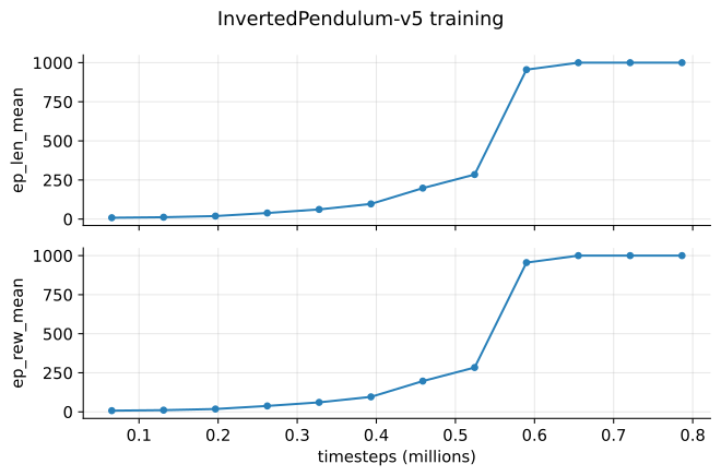
Recipe: validate PPO and its hyperparameters on a toy task first, because it separates “the algorithm is misconfigured” from “my environment is wrong”.
Learning to hover with a custom quadcopter environment
Now that we have shown that PPO plus our hyperparameters works on a toy task, let’s develop the quadcopter environment and setup a simple hover reward. We will use MuJoCo as our physics simulator.
As said in the introduction, we won’t go through all the code necessary to implement the environment, only the parts worth discussing. The rest is in src/quadcopter_racing/part_2.py.
Action design: CTBR + P controller
The policy does not directly output four motor commands. Instead, it outputs a collective thrust and body rates (CTBR) command: mass-normalized thrust and desired roll, pitch, and yaw rates. This is the action design that several papers such as Champion-level drone racing using deep reinforcement learning or Deep Drone Acrobats use. A low-level proportional (P) controller then converts this into individual motor commands, using the current body-frame angular velocity as feedback:
def _controller(
    self, omega_body: NDArray, denormalized_actions: NDArray
) -> NDArray:
    f_des = denormalized_actions[:, 0]
    w_des = denormalized_actions[:, 1:4]
    w = omega_body

    Jw = self._J_diag * w
    u_w = self._K_p * (w_des - w) + np.cross(w, Jw)

    f = f_des * self._g * self._mass / self._max_thrust / 4
    u_p, u_q, u_r = u_w[:, 0], u_w[:, 1], u_w[:, 2]

    motor = np.empty((self.num_envs, 4), dtype=np.float32)
    motor[:, 0] = f - u_p - u_q - u_r
    motor[:, 1] = f + u_p - u_q + u_r
    motor[:, 2] = f - u_p + u_q + u_r
    motor[:, 3] = f + u_p + u_q - u_r
    np.clip(motor, 0, 1, out=motor)
    return motor
CTBR is a much easier action space for the policy to learn than raw motor commands: the low-level controller handles the fast attitude-rate dynamics, while the policy reasons about thrust and desired rotation. This also helps when trying to deploy the policy on a real drone, as most controllers like Betaflight take in CTBR inputs.
The code implements a simple proportional controller, with the exception of the term np.cross(w, Jw).
To understand what it does, let’s write Euler’s rotation equation for the body-frame angular velocity \(\omega\):
The \(\omega \times J\omega\) term is the gyroscopic coupling that comes from writing the equation in a rotating (body) frame: it couples the three rotation axes together, so a pure roll rate can, through this term, generate a pitch or yaw acceleration. If we commanded torque \(\mathbf{\tau} = K_p (\omega_{des} - \omega)\) directly, this coupling term would remain in the closed-loop dynamics and distort the simple proportional response we want.
Adding it back with a + sign, u_w = K_p * (w_des - w) + np.cross(w, Jw), cancels it exactly once it is plugged back into Euler’s equation:
The two \(\omega \times J\omega\) terms cancel, resulting in a clean linear first-order response per axis. This is a small instance of feedback linearization (also called dynamic inversion): we use the known nonlinear dynamics to compute the exact torque that cancels their nonlinearity, so the remaining closed-loop system behaves like the simple linear system we designed the gain \(K_p\) for.
Recipe: have the policy output CTBR and let a P controller close the rate loop, because the controller absorbs the fast attitude dynamics and the same interface runs on real hardware.
Observation design
The observation is the 13-dimensional MuJoCo free-body state: position, attitude quaternion, linear velocity, and body-frame angular velocity.
obs[:, 0:3] = qpos[:, :3]       # position
obs[:, 3:7] = qpos[:, 3:7]      # attitude quaternion
obs[:, 7:10] = qvel[:, :3]      # linear velocity
obs[:, 10:13] = omega_body      # body-frame angular velocity
Hover reward
The reward is a potential-based progress term on the negative distance to the target, an orientation penalty, a crash penalty, and a small alive bonus:
def _reward(
    self,
    curr_obs: NDArray,
    terminated: NDArray,
) -> tuple[NDArray, NDArray]:
    pos = curr_obs[:, 0:3]
    dist = np.linalg.norm(pos - _TARGET_POS, axis=1)
    curr_potential = -dist
    progress = curr_potential - self._prev_potential

    quat_xyz = curr_obs[:, 4:7]
    orientation = -0.2 * np.linalg.norm(quat_xyz, axis=1)

    crash = np.where(terminated, -5.0, 0.0)
    alive = np.where(terminated, 0.0, 0.1)

    total = progress + orientation + crash + alive
    return total, curr_potential
Recipe: shape the reward as progress toward the target, not distance to it, because a distance penalty pays the same at every step while progress pays only for closing the gap.
Results
We trained this hover environment against three different hover targets.
For the exact hyperparameters refer to src/quadcopter_racing/part_2.py.
In all three cases, crash_rate stays around 1 for millions of steps before collapsing sharply, then distance_to_target_mean keeps decreasing for the rest of training.
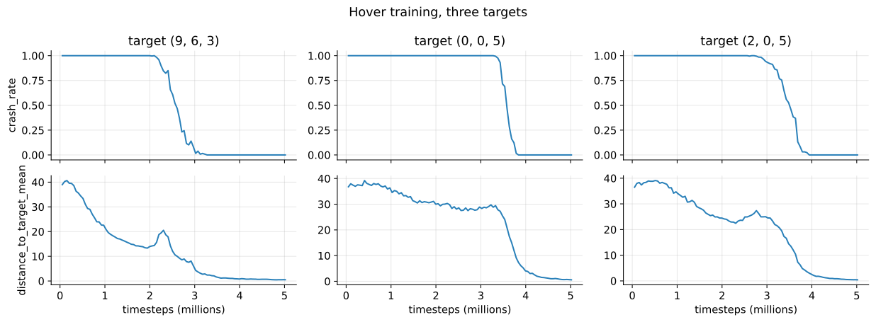
Recipe: expect
crash_rateto sit at 1 for millions of steps and then collapse, because nothing in the reward pays off until the policy can stay airborne long enough to collect it.
From hovering to racing
Hovering at a point checks that the low-level controller, reward scale, and PPO hyperparameters are implemented correctly. With that implemented and tested, we move to our next goal: racing. For that, we extend the hover environment into an eight-gate loop track.
Next gate in observation
We define two tracks: an eight-gate loop, one gate every 45 degrees around the origin at varying altitude, and a seven-gate split-S track (gate positions taken from the track.yaml released with Kaufmann et al.’s champion-level drone racing paper, dropping their orientation since our gates are point targets, not oriented rectangles).
The split-S name comes from gates 4 and 5, which sit at the same \((x, y)\) but drop from \(z=3.4\) to \(z=1.42\), forcing a steep vertical dive between them.
Regardless of the track, the position of the next gate gets appended to the observation, making the observation space 16-dimensional:
obs[:, 13:16] = target_gates
As soon as we pass a gate, the environment updates the observation. Again, for more details check out the source code, in particular: src/quadcopter_racing/part_3.py.
Next-gate reward
The reward keeps the same shape as the hover reward: progress, orientation penalty, crash penalty, alive bonus.
The only addition is a one-off bonus when the quadcopter passes within _GATE_RADIUS of the target gate, at which point the target advances to the next gate in the loop:
passed = (dist < _GATE_RADIUS) & ~terminated.astype(bool)
gate_bonus = np.where(passed, _GATE_BONUS, 0.0)

total = progress + orientation + crash + alive + gate_bonus
When a gate is passed, we also reset the potential to the new target so the progress term has no discontinuity from the target switch:
if passed.any():
    n_gates = len(self._gates)
    new_ix = (self._target_gate_indices[passed] + 1) % n_gates
    self._target_gate_indices[passed] = new_ix
    self._target_gates[passed] = self._gates[new_ix]
    curr_potential[passed] = -np.linalg.norm(
        obs[passed, 0:3] - self._target_gates[passed], axis=1
    )
    obs[passed, 13:16] = self._target_gates[passed]
    self._gates_passed_counts[passed] += 1
Random gate reset is crucial
The most important detail is how episodes reset. If every episode always spawns at gate 0, the policy must first perfect passing gate 1 before seeing gate 2 for the first time. This makes learning really hard, as the policy has very little incentive to learn how to use the target gate in its observation. Instead, every reset picks a random start gate and targets the next one in the loop:
n_gates = len(self._gates)
start_gate_ix = self._rng.integers(0, n_gates)
target_gate_ix = (start_gate_ix + 1) % n_gates
start_gate = self._gates[start_gate_ix, :]
target_gate = self._gates[target_gate_ix, :]
Recipe: randomize the start gate on every reset, because it turns one long racing task into many short one-gate tasks and forces the policy to actually read the target gate from its observation.
Results
Same environment, reward, and hyperparameters, run against both tracks.
We now also track gates_passed_mean, the mean number of gates passed per episode.
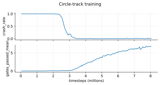
The same takeoff pattern from the hover runs shows up again: crash_rate stays around 1 for most of training, then collapses between 2.9M and 3.8M steps.
Past that point, gates_passed_mean keeps climbing steadily, reaching 3.71 gates per 400-step (8 second) episode by the end of training.
That means the converged policy isn’t just reaching one gate, it is chaining several gate passages together in a single episode, closer to the racing behavior we actually want.
The visualization at the top of the post is this converged policy, flying 24 seconds (1,200 steps) and passing 21 gates.
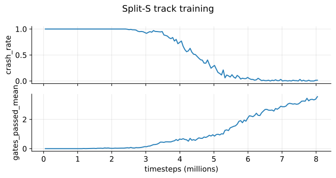
crash_rate collapses to 0 around 6.7M steps, and gates_passed_mean reaches 3.55, close to the circle track’s 3.71 at 5M steps, though the two tracks have different gate spacing so the numbers are not directly comparable.
The split-S track’s irregular gate spacing and the steep vertical dive between gates 4 and 5 don’t need a different reward or hyperparameters, just a longer takeoff window before PPO finds the working policy.
The Rerun visualization below shows the converged policy flying 24 seconds (1,200 steps), passing 12 gates despite the harder vertical maneuver between gates 4 and 5:
Takeaways and what’s next
Any complex project requires decomposing the final objective into smaller milestones, and an RL project is no different. For this specific problem, it turns out that going from toy task to hovering to racing is a nice progression. The whole post compresses to five rules:
- Validate PPO and its hyperparameters on a toy task first.
- Have the policy output CTBR and let a P controller close the rate loop.
- Shape the reward as progress toward the target, not distance to it.
- Randomize the start gate on every reset.
- Expect a long flat stretch at
crash_rate1 before anything works.
Rules 1, 4, and 5 are about the training setup rather than the vehicle, and I would reach for them on any sparse-reward control problem. Rules 2 and 3 are quadcopter specific, though the underlying moves generalize: give the policy the easiest action space that still reaches the hardware, and pay for change rather than for state. Rules 3 and 4 are the two doing the most work here, and also the two I am reporting from my own runs rather than from an ablation.
Let’s briefly discuss what the limitations currently are:
- We rely on perfect state estimation: the policy observes ground-truth position, attitude, and velocity, not sensor data like an IMU or camera. If I were to address that, I would try to re-implement “Demonstrating Agile Flight from Pixels without State Estimation”.
- Simulation only, not deployed on real hardware. I don’t own a physical drone and a racing track, but if I wanted to approach sim2real, I would start with massive domain randomization, like in “Demonstrating Agile Flight from Pixels without State Estimation”, or sim2real2sim approaches like in Champion-level drone racing using deep reinforcement learning.
- We must train for each track, and can’t zero-shot to unseen track layouts. Bridging Performance and Generalization in Reinforcement Learning for Agile Flight suggests this is tractable: they combine a procedural track generator with task switching driven by learning progress, and get a single policy that flies unseen tracks without test-time adaptation.