Simulating a 2D quadcopter from scratch
In this post, we build a simple simulation of a 2D (planar) quadcopter, a type of drone with four propellers. We will derive the equations of motion, rewrite them in state-space form, and simulate the resulting system in Python.
Why simulate a quadcopter at all? If you want to design a controller, or train a reinforcement learning agent, you first need a model you can run in software. This post builds that first simulation step from scratch in 2D, so we can understand the dynamics before moving on to control.
Problem setup and coordinates
We start with the free-body diagram shown below. We choose \(y\) as the horizontal axis and \(z\) as the vertical axis. This convention will be useful later if we extend the model to a 3D quadcopter. By the right-hand rule, the \(x\) axis points out of the page.
We model the quadcopter body as a rigid body located at \(C\) with mass \(m\) and two arms of length \(\ell\). The body can rotate in the \(yz\) plane by an angle \(\phi\). We take \(\phi > 0\) to mean a counterclockwise rotation that goes from \(y\) to \(z\). Gravity acts downward with magnitude \(mg\). Each arm carries a propeller that generates a thrust force, denoted by \(F_1\) and \(F_2\), perpendicular to the body.

Deriving the equations of motion
From this free-body diagram, we can derive the equations of motion. We begin with the Newton-Euler rigid-body equations: two translational equations, one for \(y\) and one for \(z\), and one rotational equation for \(\phi\). Here, \(F_y\) and \(F_z\) are the net force components along the corresponding axes. \(\tau\) is the net torque, and \(I\) is the moment of inertia about the center of mass. We denote time derivatives with dots, so a double dot means a second derivative with respect to time.
\[\begin{aligned} m \ddot{y} &= \sum F_y \\ m \ddot{z} &= \sum F_z \\ I \ddot{\phi} &= \sum \tau \end{aligned}\]Resolving, with some trigonometry, the thrust forces into the \(y\) and \(z\) directions gives:
\[\begin{aligned} m \ddot{y} &= - (F_1 + F_2) \sin \phi \\ m \ddot{z} &= (F_1 + F_2) \cos \phi - m g \\ I \ddot{\phi} &= (F_1 - F_2) \ell \end{aligned}\]Converting to state-space form
To simulate the system numerically, it is convenient to rewrite it in state-space form. For that, we must define the state \(\mathbf{x}\), the minimal set of variables that describes the system, and the input \(\mathbf{u}\), the variables we control. Our goal is to express how the system evolves over time in the form:
\[\mathbf{\dot{x}} = f(\mathbf{x}, \mathbf{u})\]The controllable quantities are the propeller thrusts \(F_1\) and \(F_2\). Instead of using them directly, we define the input vector as \(\mathbf{u} = \left[ (F_1 + F_2), (F_1 - F_2) \right]^T\), which leads to a cleaner formulation. Substituting these inputs into the equations of motion and isolating the derivatives on the left-hand side gives:
\[\begin{aligned} \ddot{y} &= - \frac{u_1}{m} \sin \phi \\ \ddot{z} &= \frac{u_1}{m} \cos \phi - g \\ \ddot{\phi} &= \frac{u_2}{I} \ell \end{aligned}\]Because standard state-space models are first order, we introduce the state vector:
\[\mathbf{x} = \left[ y, z, \phi, \dot{y}, \dot{z}, \dot{\phi} \right]^T\]By including the velocities in the state, we can write the full first-order system as:
\[\mathbf{\dot{x}} = \begin{bmatrix} \dot{y} \\ \dot{z} \\ \dot{\phi} \\ \ddot{y} \\ \ddot{z} \\ \ddot{\phi} \end{bmatrix} = f(\mathbf{x}, \mathbf{u}) = \begin{bmatrix} \dot{y} \\ \dot{z} \\ \dot{\phi} \\ - \frac{u_1}{m} \sin \phi \\ \frac{u_1}{m} \cos \phi - g \\ \frac{u_2}{I} \ell \end{bmatrix}\]Simulating the system in Python
We can now simulate this state-space model in Python. First, we define the physical parameters and the dynamics function:
import numpy as np
from numpy.typing import NDArray

m = 0.8  # [kg]
g = 9.81  # [m/s^2]
l = 0.5  # [m]
I = 1e-3  # [kg*m^2]


def dynamics(x: NDArray, u: NDArray) -> NDArray:
    _y, _z, phi, y_dot, z_dot, phi_dot = x
    return np.array(
        [
            y_dot,
            z_dot,
            phi_dot,
            -u[0] / m * np.sin(phi),
            u[0] / m * np.cos(phi) - g,
            u[1] / I * l,
        ]
    )
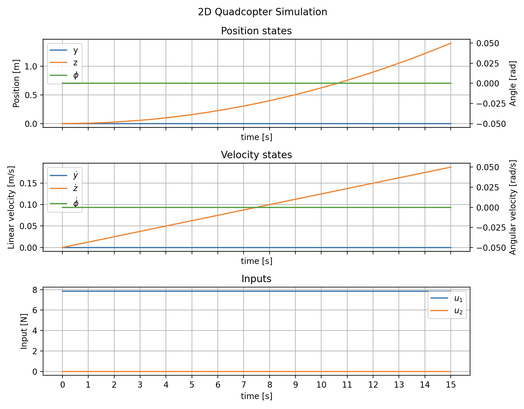
With the dynamics defined, we solve the first-order ordinary differential equation with Euler’s method to calculate the full trajectory. We initialize the state at zero, so the quadcopter starts at the origin with no velocity and no rotation. We choose a constant input \(u_1 = F_1 + F_2 = mg + 0.01\) so the quadcopter produces slightly more thrust than its weight and slowly ascends. We set \(u_2 = 0\) so there is no net torque and the vehicle does not rotate.
t_start, t_stop, n_steps = 0.0, 15.0, 1_000
t = np.linspace(start=t_start, stop=t_stop, num=n_steps)
dt = t[1] - t[0]

d_state = 6
x = np.zeros(shape=(n_steps, d_state))

d_input = 2
u = np.zeros(shape=(n_steps, d_input))
u[:, 0] = m * g + 0.01  # Enough thrust to beat gravity plus a bit more.

for i in range(n_steps - 1):
    x[i + 1] = x[i] + dynamics(x[i], u[i]) * dt
That is the complete simulation pipeline: derive the equations of motion, convert them to state-space form, and integrate them numerically in Python.
Running the simulation
Zero-torque case
We confirm that our simulation performs as expected with the plot shown below. As expected, the \(y\) position and \(\phi\) angle stay constant, as well as their respective velocities \(\dot{y}\) and \(\dot{\phi}\). In this constant-input, zero-torque case, the vertical acceleration is constant, so the \(z\) position grows quadratically and the \(\dot{z}\) velocity grows linearly.
In addition to the static plots, I implemented a small visualizer that animates the quadcopter in the \(yz\) plane using the simulated state trajectory.
Simulation visualizer
Non-zero torque case
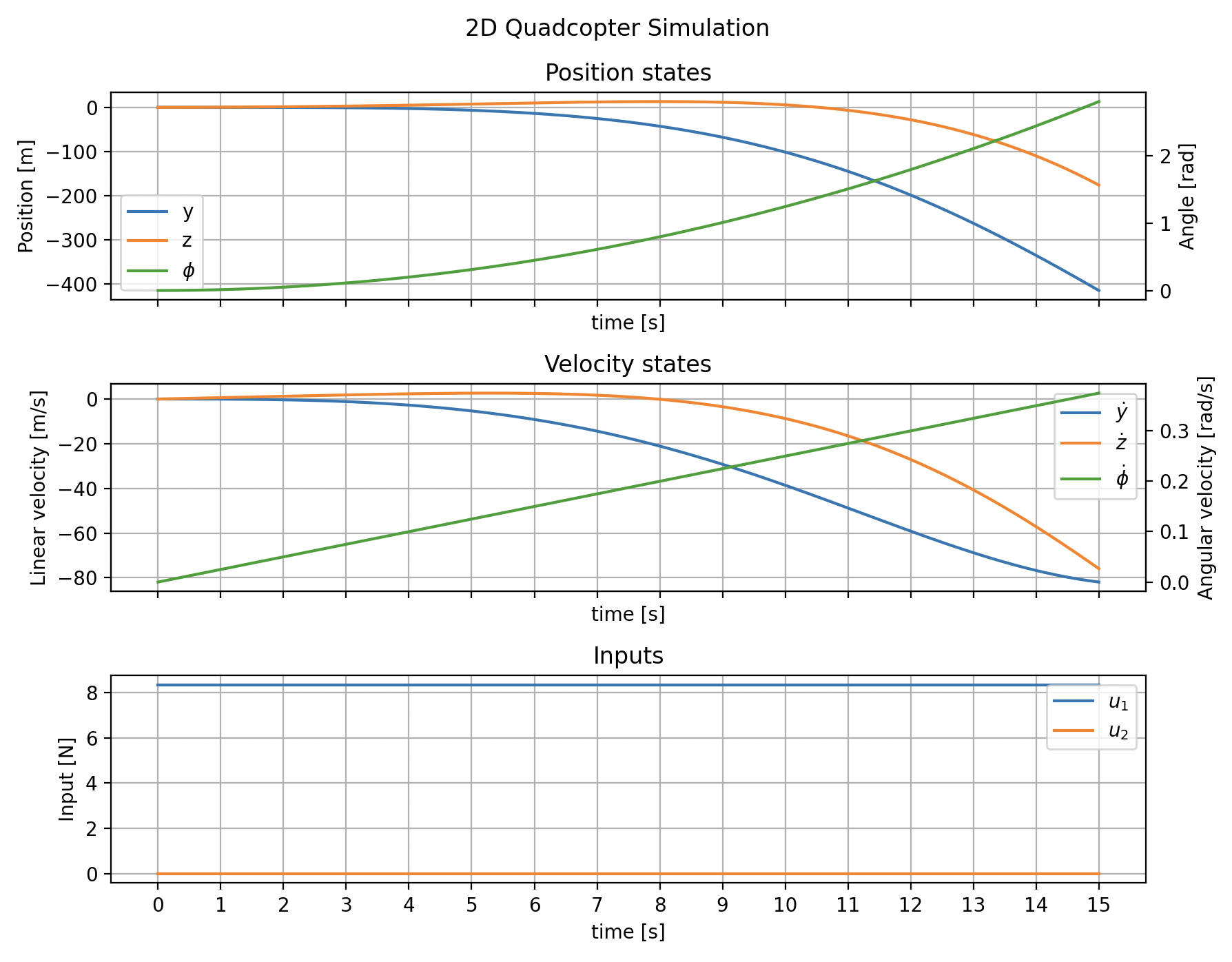
Let’s now apply a nonzero torque input \(u_2\) and also increase the total thrust \(u_1\). Since this simple model does not include ground contact, we stop the simulation once the quadcopter crosses below \(z = 0\), which we treat as ground level:
d_input = 2
u = np.zeros(shape=(n_steps, d_input))
u[:, 0] = m * g + 0.5
u[:, 1] = 5e-5

eps = 1e-8
for i in range(n_steps - 1):
    if x[i, 1] < -eps:  # Quadcopter crashes, stop the simulation.
        t = t[:i]
        x = x[:i, :]
        u = u[:i, :]
        break
    x[i + 1] = x[i] + dynamics(x[i], u[i]) * dt
And running the simulation gives us the plot below. The angle slowly increases from 0 to approximately 3 radians, so the quadcopter rotates until it is nearly upside down. It gains height initially, but as \(\phi\) increases, the vertical acceleration \(\ddot{z} = \frac{u_1}{m}\cos\phi - g\) decreases because the vertical component of thrust shrinks. Once \(\frac{u_1}{m}\cos\phi < g\), gravity dominates and the quadcopter starts falling.
Simulation visualizer
Note about LLM usage: This post was written fully by a human and proofread and minimally edited by gpt-5.4 default (via codex).
Appendix: plotting code
import matplotlib.pyplot as plt  # noqa: E402
from matplotlib.ticker import MultipleLocator  # noqa: E402

fig, axes = plt.subplots(nrows=3, sharex=True, figsize=(9, 7))

ax0, ax0r = axes[0], axes[0].twinx()
ax0.plot(t, x[:, 0], label="y", color="C0")
ax0.plot(t, x[:, 1], label="z", color="C1")
ax0r.plot(t, x[:, 2], label="$\\phi$", color="C2")
ax0.set_ylabel("Position [m]")
ax0r.set_ylabel("Angle [rad]")
ax0.set_title("Position states")
lines0 = ax0.get_lines() + ax0r.get_lines()
ax0.legend(handles=lines0, labels=[line.get_label() for line in lines0])

ax1, ax1r = axes[1], axes[1].twinx()
ax1.plot(t, x[:, 3], label="$\\dot{y}$", color="C0")
ax1.plot(t, x[:, 4], label="$\\dot{z}$", color="C1")
ax1r.plot(t, x[:, 5], label="$\\dot{\\phi}$", color="C2")
ax1.set_ylabel("Linear velocity [m/s]")
ax1r.set_ylabel("Angular velocity [rad/s]")
ax1.set_title("Velocity states")
lines1 = ax1.get_lines() + ax1r.get_lines()
ax1.legend(handles=lines1, labels=[line.get_label() for line in lines1])

axes[2].plot(t, u[:, 0], label="$u_1$")
axes[2].plot(t, u[:, 1], label="$u_2$")
axes[2].set_title("Inputs")
axes[2].set_ylabel("Input [N]")
axes[2].legend()

for ax in axes:
    ax.xaxis.set_major_locator(MultipleLocator(1))
    ax.set_xlabel("time [s]")
    ax.grid(visible=True)

fig.suptitle("2D Quadcopter Simulation")
fig.tight_layout()
plt.show()