Simulating a 3D quadcopter from scratch
This post is the second post in our series on quadcopter simulation. If you want the simpler planar version first, the previous post derives and simulates the same ideas in 2D, but this post is fully standalone. Today, we simulate a three-dimensional quadcopter. We will derive the equations of motion, transform them into state-space form, and finally simulate the system in Python. Along the way, we introduce quaternions and quaternion derivatives.
Problem setup and coordinates
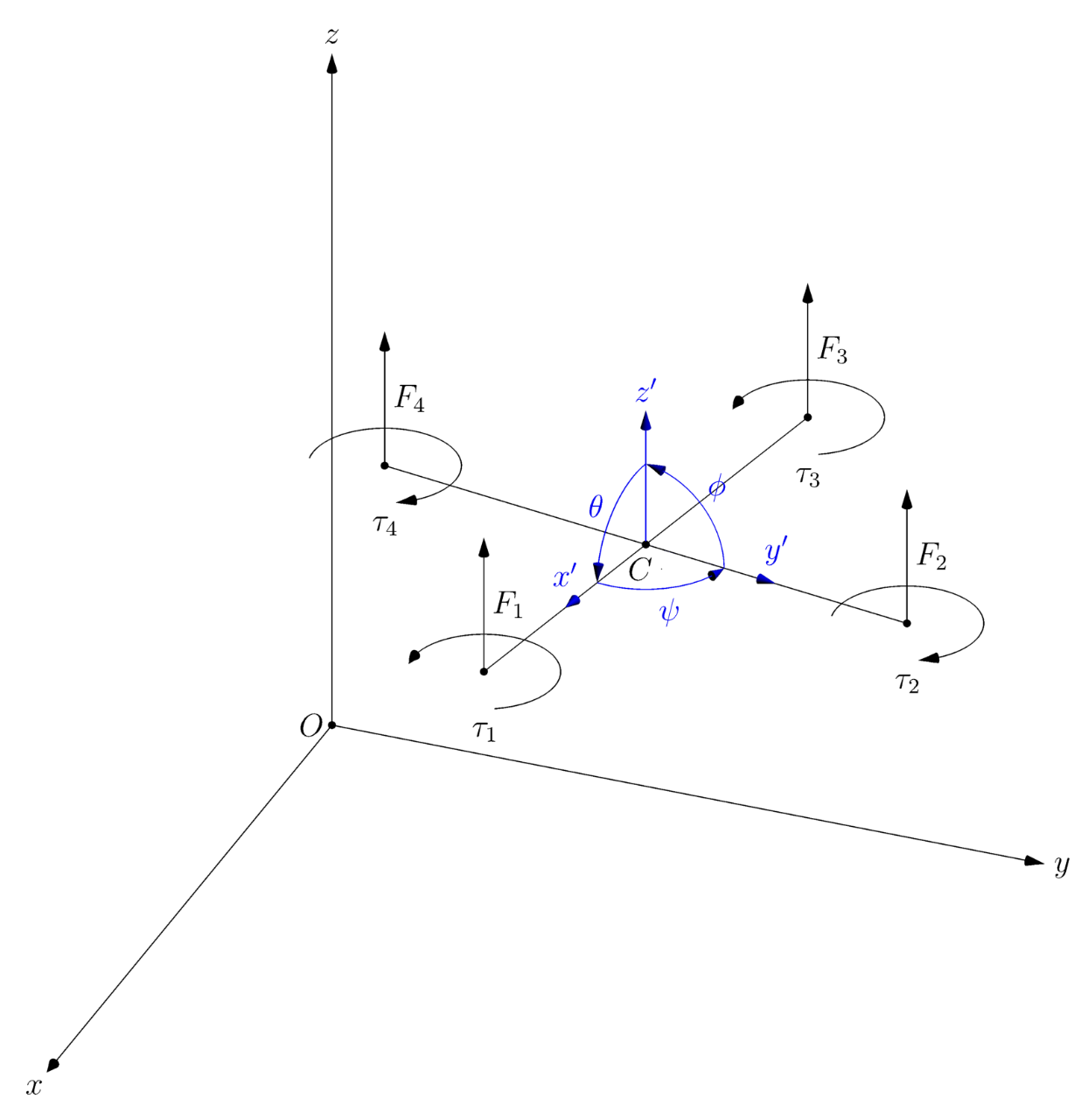
The free-body diagram for the quadcopter is shown below. We use a right-hand coordinate frame with the \(z\) axis for altitude. The axes \(\{x, y, z\}\) are constant over time and form the world frame. This frame of reference is inertial (does not accelerate). The axes \(\{x', y', z'\}\) instead are always attached to the quadcopter center of mass and form the body frame, which changes over time. The body frame is not an inertial frame of reference, as the drone accelerates. Some equations of motion are easier to write in the world frame while others in the body frame. Our model uses both.
The quadcopter is made of four rods of length \(\ell\) laid in a “+” pattern around the center \(C\). There is a spinning propeller at the end of each rod, which generates thrust \(F_i\). Propeller drag generates a torque \(\tau_{i} = \frac{F_i}{k}\) opposite to the propeller spin direction. The quadcopter can have arbitrary position and attitude (i.e. its orientation). Let \(\mathbf{p}\) be the position vector from origin \(O\) to center of mass \(C\). Let \(q\) be the quaternion that rotates a vector’s coordinates from the body frame to the world frame, representing the attitude.
Quaternions
We briefly introduce quaternions here because they are the most convenient way to represent attitude in this model. Quaternions, unit quaternions to be precise, are a way to represent rotations. Rotations, especially in 3D, are strange objects as they don’t live in the usual \(\mathbb{R}^3\) like position or velocity vectors. Instead, rotations live in a space called the 3D special orthogonal group, or \(\text{SO}(3)\). Representing \(\text{SO}(3)\) objects in \(\mathbb{R}^3\) is possible, for example using Euler angles, but leads to issues like singularities and numerical instability. For our purposes, representing attitude with quaternions leads to simpler, more efficient, and more numerically stable code. For a geometric introduction to quaternions, I recommend this video by Freya Holmer. We’ll talk more about quaternions, specifically about their derivatives, later in the post.
Deriving the equations of motion
To simulate the quadcopter, we need a differential equation that tells us how its state changes under a given motor input. That starts with the rigid-body equations of motion: once we know the translational and rotational accelerations, we can package them into a first-order state-space model and integrate it numerically.
Having introduced our free body diagram, let’s write the Newton-Euler rigid body equations of motion. In 2D we could work with three scalar equations, two for position (\(y, z\) axes) and one for rotation. In 3D we have six equations: three for translation (in world frame), three for rotation (in body frame), written in vector form. \(\mathbf{\dot{v}}\) is the time derivative of velocity, itself the derivative of position \(\mathbf{p}\). \(\dot{\omega}\) is the time derivative of angular velocity, which is not the derivative of attitude (the two are connected via the kinematic matrix). Finally, \(m\) is the mass and \(I\) is the moment of inertia.
\[\begin{aligned} m \mathbf{\dot{v}} &= \sum_i \mathbf{F_i} && \text{(world frame)} \\ I \dot{\omega} + \omega \times I \omega &= \sum_i \mathbf{\tau_i} && \text{(body frame)} \end{aligned}\]Let’s now plug in the forces from the free-body diagram into the translation equations. In world frame where the axes are \(\{x, y, z\}\), our quadcopter is subject to the gravitational force \(-m\mathbf{g}\) where \(\mathbf{g} = \left[0, 0, g\right]^T_{\text{world}}\). Additionally, each motor produces thrust \(\mathbf{F_i}\) of magnitude \(F_i\), but this vector is only easy to write in body frame, where the motors always point straight up: \(\mathbf{F_i} = \left[0, 0, F_i\right]^T_{\text{body}}\). To convert our simple expression for thrusts from body frame into world frame, we must rotate them. To rotate the body frame vector to world frame we use the attitude quaternion \(q\).
We derive the rotation equations in the body frame by seeing how each force or torque affects each rotation axis. We denote rotations about the body-frame axes by roll \(\phi\), pitch \(\theta\), and yaw \(\psi\). If the second motor speeds up, increasing \(F_2\), roll \(\phi\) will increase. If the fourth motor speeds up, increasing \(F_4\), roll \(\phi\) will decrease. Thus the force couple \((F_2 - F_4)\), multiplied by arm length \(\ell\), will form the torque on the \(x'\) axis. The same argument holds for \(F_1, F_3\) and \(\theta\) (pitch) on the \(y'\) axis. Finally, for \(\psi\) (yaw) on the \(z'\) axis, we simply add together all propeller drag torques \(\tau_i\) (positive sign for CCW rotation, negative for CW).
\[\begin{aligned} m \mathbf{\dot{v}} &= -m\mathbf{g} + \text{rotate}(q, \sum_i \mathbf{F_i}) \\ I \dot{\omega} + \omega \times I \omega &= \begin{bmatrix} \ell (F_2 - F_4) \\ \ell (F_3 - F_1) \\ \tau_1 - \tau_2 + \tau_3 - \tau_4 \end{bmatrix} \end{aligned}\]At this point we have expressions for translational acceleration \(\mathbf{\dot{v}}\) and angular acceleration \(\dot{\omega}\) in terms of thrusts and attitude. To get to a simulator, two pieces are still missing: the kinematics that connect these accelerations back to the state variables, and a mapping from control inputs to the four motor thrusts \(F_i\).
Converting to state-space form
Let’s now start re-arranging the equations so that we can write our system in state-space form. First, let’s define mass-normalized thrust \(\mathbf{c}\) and torques \(\mathbf{\Tau}\):
\[\begin{aligned} \mathbf{c} &= \frac{1}{m} (\mathbf{F_1} + \mathbf{F_2} + \mathbf{F_3} + \mathbf{F_4}) \\ \mathbf{\Tau} &= \begin{bmatrix} \ell (F_2 - F_4) \\ \ell (F_3 - F_1) \\ \tau_1 - \tau_2 + \tau_3 - \tau_4 \end{bmatrix} \end{aligned}\]With these defined, we isolate the derivatives of (linear) velocity and angular velocity on the left-hand side:
\[\begin{aligned} \mathbf{\dot{v}} &= -\mathbf{g} + \text{rotate}(q, \mathbf{c}) \\ \dot{\omega} &= I^{-1} (\mathbf{\Tau} - \omega \times I \omega) \end{aligned}\]Our goal is to express how the system evolves over time in the form:
\[\mathbf{\dot{x}} = f(\mathbf{x}, \mathbf{u})\]We describe later how the input \(\mathbf{u}\) is parametrized, so for now we focus on the state and leave the force terms abstract. We want a first-order system, so we include velocities \(\mathbf{v}\) and \(\omega\) in the state. But what should our zeroth-order quantities be? For translations, it’s easy, we will use position \(\mathbf{p}\) whose derivative is the velocity. For rotations, it turns out that the best parametrization is the quaternion \(q\). This results in a \(13\)-dimensional \((3 + 4 + 3 + 3)\) state:
\[\mathbf{x} = \left[\mathbf{p}, q, \mathbf{v}, \omega \right]^T\]Which we use to write our system as:
\[\mathbf{\dot{x}} = \begin{bmatrix} \mathbf{\dot{p}} \\ \dot{q} \\ \mathbf{\dot{v}} \\ \dot{\omega} \end{bmatrix} = f(\mathbf{x}, \mathbf{u}) = \begin{bmatrix} \mathbf{v} \\ ? \\ -\mathbf{g} + \text{rotate}(q, \mathbf{c}) \\ I^{-1} (\mathbf{\Tau} - \omega \times I \omega) \end{bmatrix}\]The only missing row is the quaternion derivative \(\dot{q}\). The only remaining step is to specify how the input \(\mathbf{u}\) determines \(\mathbf{c}\) and \(\mathbf{\Tau}\).
Quaternion derivatives
We now need an expression for the derivative of the attitude quaternion. A fully rigorous treatment takes us beyond the scope of this post, so we derive the formula in the form needed for the simulator. The argument below follows Quaternion differentiation, adapted to this post’s notation.
Let \(q(0) = q\) be our attitude quaternion at time \(t=0\). We denote quaternion multiplication between quaternions \(q_a\) and \(q_b\) with \(q_a \otimes q_b\). Our quadcopter rotates with angular velocity \(\omega\), so over one unit of time it rotates by \(\omega\) (treating \(\omega\) as instantaneous). Let \(q_{\omega}\) be the quaternion representing the rotation. This means that at time \(t = 1\), we have \(q(1) = q \otimes q_{\omega}\) (notice how the transformation is applied on the right). And, by induction, \(q(t) = q \otimes q_{\omega}^t\) at time \(t\) (this is only true for small, instantaneous time steps as \(\omega\) itself changes through time).
Any unit quaternion can be represented as the exponential of a pure imaginary quaternion, just like any complex number \(z\) can be written as the exponential of a pure imaginary number \(i\theta\) or \(z = e^{i\theta}\). We call \(\omega^{\wedge}\) the pure imaginary quaternion (a 4D quantity) created from the 3D angular velocity \(\omega\) (in the body frame), that is \(\omega^{\wedge} = \left(0, \omega_1, \omega_2, \omega_3 \right)\). This lets us write \(q_{\omega} = e^{\frac{1}{2} \omega^{\wedge}}\) and \(q_{\omega}^t = e^{\frac{1}{2} \omega^{\wedge} t}\). The additional factor \(\frac{1}{2}\) is a result of how quaternions are a “double cover” of rotations, an artifact of the particular representation of \(\text{SO}(3)\) we picked.
With these definitions, we can write
\[q(t) = q \otimes e^{\frac{1}{2} \omega^{\wedge} t}\]Differentiating with respect to time gives
\[\begin{aligned} \dot{q}(t) &= q \otimes e^{\frac{1}{2} \omega^{\wedge} t} \otimes \frac{1}{2} \omega^{\wedge} \\ \dot{q}(t) &= q(t) \otimes \frac{1}{2} \omega^{\wedge} \end{aligned}\]With this expression for \(\dot{q}\), we can complete the state-space formulation of the system:
\[\mathbf{\dot{x}} = \begin{bmatrix} \mathbf{\dot{p}} \\ \dot{q} \\ \mathbf{\dot{v}} \\ \dot{\omega} \end{bmatrix} = f(\mathbf{x}, \mathbf{u}) = \begin{bmatrix} \mathbf{v} \\ q \otimes \frac{1}{2} \omega^{\wedge} \\ -\mathbf{g} + \text{rotate}(q, \mathbf{c}) \\ I^{-1} (\mathbf{\Tau} - \omega \times I \omega) \end{bmatrix}\]Input parameter and mixer equations
The last piece we need is how to parametrize our inputs \(\mathbf{u}\) and how they translate into our forces \(F_i\). This choice is a bit arbitrary, but following Deep Drone Acrobatics and Champion-level drone racing using deep reinforcement learning we use mass-normalized thrust and three rotational control inputs. We call the inputs \(u_c\) for mass-normalized thrust and \(u_p, u_q, u_r\) for roll, pitch, and yaw control. The function mapping inputs to forces is called “mixer”. For more details on how to extend this to more shapes and propellers check out Motor Mixer Theory. We omit the derivation, which is a simple geometric argument from the free body diagram.
Let \(F_t = \frac{u_c m}{4}\), with \(k\) the propeller-drag ratio, then our mixer is:
\[\begin{aligned} \begin{bmatrix} F_1 \\ F_2 \\ F_3 \\ F_4 \end{bmatrix} = \text{mixer}\left( \begin{bmatrix} u_c \\ u_p \\ u_q \\ u_r \end{bmatrix} \right) \\ = \begin{bmatrix} F_t - u_q / 2\ell + u_r / 4k \\ F_t + u_p / 2\ell - u_r / 4k \\ F_t + u_q / 2\ell + u_r / 4k \\ F_t - u_p / 2\ell - u_r / 4k \end{bmatrix} \end{aligned}\]Substituting these four thrusts into \(\mathbf{c}\) and \(\mathbf{\Tau}\) gives a fully specified system \(\mathbf{\dot{x}} = f(\mathbf{x}, \mathbf{u})\).
Simulating the system in Python
We can now simulate the system in Python. First, we define the physical parameters, the dynamics function, and the mixer function. Code for the quaternion utility functions we use is in the appendix.
g = 9.81  # [m/s^2] gravity
m = 0.8  # [kg] mass
L = 0.5  # [m] arm length
k = 100  # [] thrust / drag ratio.
I = np.diag([0.001, 0.001, 0.002])  # noqa: E741  # inertia matrix.
I_inv = np.linalg.inv(I)


def dynamics(x: NDArray, u: NDArray) -> NDArray:
    F1, F2, F3, F4 = mixer(u)

    q, v, omega = x[3:7], x[7:10], x[10:13]
    c = np.array([0, 0, (F1 + F2 + F3 + F4) / m])
    tau1, tau2, tau3, tau4 = F1 / k, F2 / k, F3 / k, F4 / k
    Tau = np.array([L * (F2 - F4), L * (F3 - F1), tau1 - tau2 + tau3 - tau4])

    return np.concat(
        [
            v,
            0.5 * quat_mul(q, np.array([0, *omega])),
            np.array([0, 0, -g]) + rot_vec_by_quat(q, c),
            I_inv @ (Tau - np.cross(omega, I @ omega)),
        ]
    )

def mixer(u: NDArray) -> NDArray:
    u_c, u_p, u_q, u_r = u
    F_t = u_c * m / 4
    F1 = F_t - u_q / (2 * L) + u_r / (4 * k)
    F2 = F_t + u_p / (2 * L) - u_r / (4 * k)
    F3 = F_t + u_q / (2 * L) + u_r / (4 * k)
    F4 = F_t - u_p / (2 * L) - u_r / (4 * k)
    return np.array([F1, F2, F3, F4])
With the dynamics (and mixer) defined, we use Euler’s method to solve the first-order ordinary differential equations. We initialize the quadcopter two meters above the origin at \(\mathbf{p}=(0, 0, 2)\). A “zero” rotation is a unit quaternion \((1, 0, 0, 0)\). We set the mass-normalized thrust \(u_c\) to be just above \(g\), so the quadcopter accelerates upward. We set the yaw control input \(u_r\) to a piecewise-constant function: it is 0 at first, then 10 for one second, then 0 for one second, then -10 for one second, and finally 0 again.
t_start = 0.0
t_stop = 10.0
n_steps = 10_000
t = np.linspace(t_start, t_stop, n_steps)
dt = t[1] - t[0]

d_state = 13  # 13 = 3 (position) + 4 (attitude quaternion) + 3 (velocity) + 3 (body rate).
x = np.zeros((n_steps, d_state))
x[0, 2] = 2  # start at z=2
x[0, 3:7] = np.array([1, 0, 0, 0])  # initialize quaternion to unit length.

d_input = 4
u = np.zeros((n_steps, d_input))
u[:, 0] = 9.81 + 0.05
u[:, 3] = 10 * (
    np.heaviside(t - 1, 1)
    - np.heaviside(t - 2, 1)
    - np.heaviside(t - 3, 1)
    + np.heaviside(t - 4, 1)
)

for i in range(n_steps - 1):
    x[i + 1, :] = x[i, :] + dynamics(x[i], u[i]) * dt

    # Quaternion drifts under Euler integration, so we renormalize it.
    q = x[i + 1, 3:7]
    x[i + 1, 3:7] = q / np.linalg.norm(q)
That is the complete simulation pipeline: derive the equations of motion, convert them to state-space form, and integrate them numerically in Python.
Running the simulation
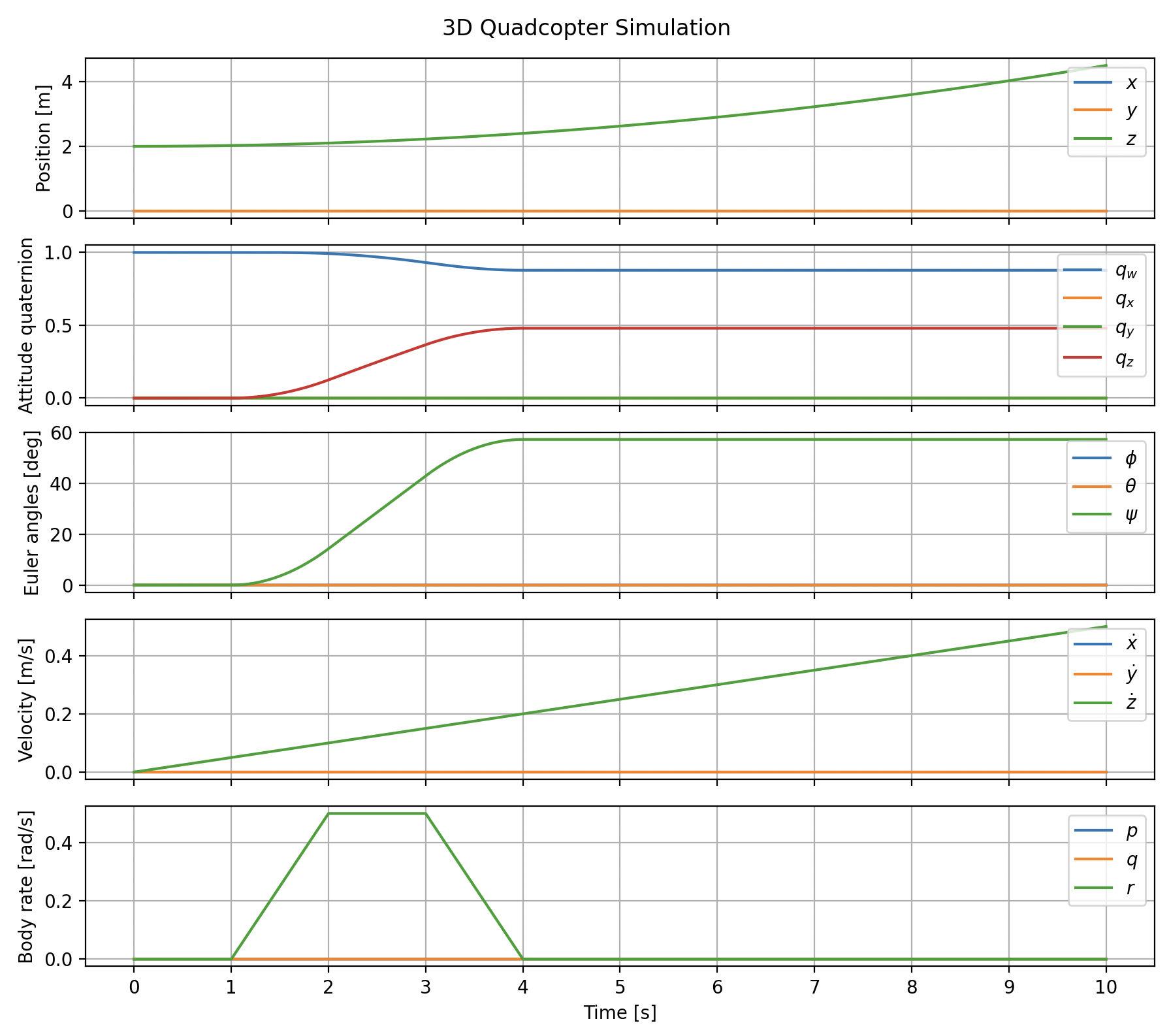
Upwards acceleration and yaw input
We run the simulation with the input parameters described above and check that it performs as expected. The quadcopter’s position does not change in \(x\) or \(y\), but the \(z\) coordinate increases as thrust is greater than gravitational acceleration. The stepwise yaw control causes yaw (\(\psi\)) to start at zero and grow to \(\approx 60^{\circ}\). The body rates are labeled \((p, q, r)\), the conventional names for the body-frame angular velocity components \(\omega_{x'}, \omega_{y'}, \omega_{z'}\).
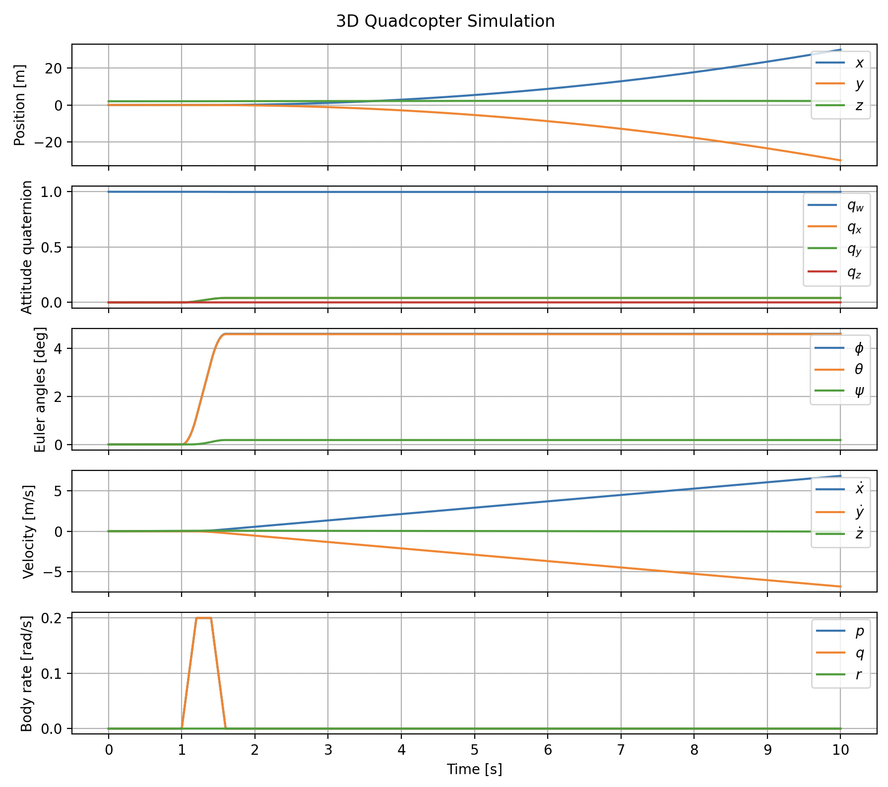
Translation via pitch and roll input
To move the quadcopter horizontally, we tilt it: a non-zero roll or pitch points the thrust vector away from the world \(z\) axis, leaving an unbalanced horizontal component that accelerates the body. We apply equal, brief pulses to the roll and pitch inputs \(u_p\) and \(u_q\): a positive pulse between \(t=1.0\) and \(t=1.2\), then a negative pulse between \(t=1.4\) and \(t=1.6\). Mass-normalized thrust \(u_c\) is held just above \(g\) as before, and yaw input \(u_r\) is zero throughout.
u = np.zeros((n_steps, d_input))
u[:, 0] = 9.81 + 0.05
u[:, 1] = u[:, 2] = 1e-3 * (
    np.heaviside(t - 1.0, 1)
    - np.heaviside(t - 1.2, 1)
    - np.heaviside(t - 1.4, 1)
    + np.heaviside(t - 1.6, 1)
)
The plot below confirms the expected behavior. The body rates \(p\) and \(q\) show the input pulse and then return to zero, leaving roll \(\phi\) and pitch \(\theta\) tilted at a few degrees each. With no restoring torque in this open-loop system, the attitude stays tilted for the rest of the simulation. The tilted thrust vector then accelerates the quadcopter linearly: \(\dot{x}\) grows positive and \(\dot{y}\) grows negative, producing the linear drift in \(x\) and \(y\) position. The \(z\) coordinate barely changes, since the vertical component of thrust, scaled by \(\cos\phi \cos\theta\), remains close to \(g\) at small tilt angles.
The Rerun visualization below shows the same trajectory in 3D, making it easier to see how a brief tilt input leads to persistent sideways drift in open loop.
Note about LLM usage: This post was written fully by a human and proofread and minimally edited by gpt-5.4 medium (via codex) and Opus 4.7 medium effort (via Claude).
Appendix: quaternion utility functions
def rot_vec_by_quat(q: NDArray, v: NDArray) -> NDArray:
    w = q[0]
    q_vec = q[1:4]
    t = 2.0 * np.cross(q_vec, v)
    return v + w * t + np.cross(q_vec, t)


def quat_mul(p: NDArray[np.float64], q: NDArray[np.float64]) -> NDArray[np.float64]:
    pw, px, py, pz = p
    qw, qx, qy, qz = q

    r = np.empty(4, dtype=np.float64)

    r[0] = pw * qw - px * qx - py * qy - pz * qz
    r[1] = pw * qx + px * qw + py * qz - pz * qy
    r[2] = pw * qy - px * qz + py * qw + pz * qx
    r[3] = pw * qz + px * qy - py * qx + pz * qw

    return r
Appendix: plotting code
def quaternion_to_euler(q: NDArray) -> tuple[float, float, float]:
    w, qx, qy, qz = q
    phi = np.arctan2(2 * (w * qx + qy * qz), 1 - 2 * (qx**2 + qy**2))
    theta = np.arcsin(2 * (w * qy - qz * qx))
    psi = np.arctan2(2 * (w * qz + qx * qy), 1 - 2 * (qy**2 + qz**2))
    return float(phi), float(theta), float(psi)


euler = np.array([quaternion_to_euler(x[i, 3:7]) for i in range(n_steps)])

fig, axes = plt.subplots(5, 1, figsize=(9, 8), sharex=True)

for i, name in enumerate(["$x$", "$y$", "$z$"]):
    axes[0].plot(t, x[:, i], label=name)
axes[0].set_ylabel("Position [m]")
axes[0].legend(loc="upper right")
axes[0].grid(visible=True)

for i, name in enumerate(["$q_w$", "$q_x$", "$q_y$", "$q_z$"]):
    axes[1].plot(t, x[:, 3 + i], label=name)
axes[1].set_ylabel("Attitude quaternion")
axes[1].legend(loc="upper right")
axes[1].grid(visible=True)

for i, name in enumerate(["$\\phi$", "$\\theta$", "$\\psi$"]):
    axes[2].plot(t, np.rad2deg(euler[:, i]), label=name)
axes[2].set_ylabel("Euler angles [deg]")
axes[2].legend(loc="upper right")
axes[2].grid(visible=True)

for i, name in enumerate(["$\\dot{x}$", "$\\dot{y}$", "$\\dot{z}$"]):
    axes[3].plot(t, x[:, 7 + i], label=name)
axes[3].set_ylabel("Velocity [m/s]")
axes[3].legend(loc="upper right")
axes[3].grid(visible=True)

for i, name in enumerate(["$p$", "$q$", "$r$"]):
    axes[4].plot(t, x[:, 10 + i], label=name)
axes[4].set_ylabel("Body rate [rad/s]")
axes[4].legend(loc="upper right")
axes[4].grid(visible=True)

axes[4].set_xlabel("Time [s]")
axes[4].xaxis.set_major_locator(plt.MultipleLocator(1))

fig.suptitle("3D Quadcopter Simulation")
fig.tight_layout()
plt.show()