One Dimensional Variational Inference
In this post we will get our hands dirty and use the concepts we learned in “What is the ELBO in Variational Inference?” to perform variational inference for a 1D distribution.
As this post is a Jupyter notebook, we first begin with the usual scientific Python imports.
import numpy as np
import seaborn as sns
import matplotlib.pyplot as plt
%config InlineBackend.figure_format='retina'
sns.set_theme(style='darkgrid')

from scipy.stats import norm, skewnorm
from scipy.optimize import minimize
from scipy.integrate import quad
Prior, likelihood, and posterior
We begin by implementing the prior and the likelihood. The prior is a Normal distribution centered around 0 and with standard deviation 5. We make the standard deviation large to allow for a wide range posterior values. The likelihood, thanks to Variational Inference, can be any distribution, since we don’t need the prior and likelihood to be conjugate. We chose the likelihood to have the PDF of a skew normal distribution.
PRIOR_MU = 0
PRIOR_SIGMA = 5


def prior(theta):
    "p(theta) = N(theta | 0, 5)"
    return norm.pdf(theta, loc=PRIOR_MU, scale=PRIOR_SIGMA)


def likelihood(y, theta):
    "p(y | theta) = skewnorm(y | 5, theta, 2)"
    return skewnorm.pdf(y, a=5, loc=theta, scale=2)
We numerically compute our posterior as there is no analytical solution for it. This is possible because we are in 1D but for real-world high-dimensional problems, this is untractable. We will use it to verify the correctness of our solution.
def posterior(theta, y):
    "p(theta | y) = p(y | theta) * p(theta) / p(y)"
    evidence, _ = quad(
        lambda theta_: likelihood(y, theta_) * prior(theta_),
        -np.inf,
        np.inf,
    )
    return likelihood(y, theta) * prior(theta) / evidence
Variational posterior and variational objective
And now to the juicy parts: we need to implement our variational posterior and the variational objective that we will maximize. We choose the variational posterior to be Normal as it is a flexible distribution and it gives us a closed-form expression for the KL-divergence of the variational posterior and prior. The variational objective uses numerical integration to compute the 1D integrals of the data fit term and closed-form expression for the KL divergence. Even if we were solving this problem in higher dimensions, the data fit term will be a product of 1D integrals, which is a bit more expensive to compute but its complexity is linear in the number of dimensions, not exponential.
def variational_posterior(theta, m, s):
    "q(theta) = N(theta | m, s))"
    return norm.pdf(theta, loc=m, scale=s)


def data_fit_term(y, m, s):
    "E_q(theta | m, s) [log p(y | theta)]"
    integral, _ = quad(
        lambda theta: variational_posterior(theta, m, s)
        * (np.log(likelihood(y, theta) + 1e-8)),
        -np.inf,
        np.inf,
    )
    return integral


def kl_term(m, s):
    "KL(q(theta | m, s) || p(theta))"
    return np.log(PRIOR_SIGMA / s) + (
        (s**2 + (m - PRIOR_MU) ** 2) / (2 * PRIOR_SIGMA**2) - 0.5
    )


def variational_objective(y, m, s):
    return data_fit_term(y, m, s) - kl_term(m, s)
Finding the best variational approximation
Before solving our optimization problem, let’s first see what our starting state looks like with the plotting function defined below.
def plot_variational_and_true_posterior(y, theta, m, s):
    fig, ax = plt.subplots(figsize=(8, 4))

    ax.plot(theta, prior(theta), label="$p(\\theta)$")
    ax.plot(theta, variational_posterior(theta, m, s), label="$q(\\theta)$")
    ax.plot(theta, posterior(theta, y), label="$p(\\theta | y)$")

    ax.set_xlabel("$\\theta$")
    ax.set_ylabel("Density")

    obj = variational_objective(y, m, s)

    ax.set_title(
        f"""
Prior, variational posterior, and true posterior
$m$={m:.2f}, $s$={s:.2f}, $L[q]$={obj:.2f}
    """
    )
    ax.legend()

    fig.tight_layout()
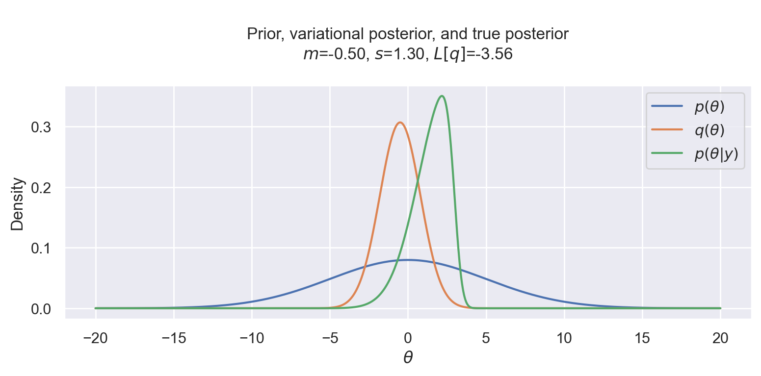
We assume that our only observation is y=3 and we plot the prior, variational posterior, and true posterior for a range of values.
y = 3
theta = np.linspace(-20, 20, 1000)
plot_variational_and_true_posterior(y, theta, -0.5, 1.3)
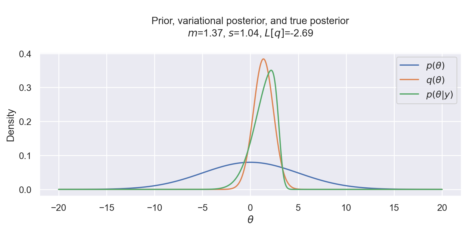
Now we can finally run Scipy’s optimizer to maximize (or minimize the negated) variational objective. And see that it indeed worked! The variational posterior is quite close to the true posterior distribution. We can also see that the normal variational posterior is not skewed like the likelihood, but it tries to compensate by moving the mean to the left, where the posterior is skewed.
res = minimize(
    lambda x: -variational_objective(y, x[0], x[1]),
    x0=[0, 5],
    bounds=[(-10, 10), (0.1, 10)],
)
m, s = res.x
plot_variational_and_true_posterior(y, theta, m, s)
That’s all folks! In the next post we will run a similar experiment, but using multiple dimensions.