The Volatility Smile

Introduction

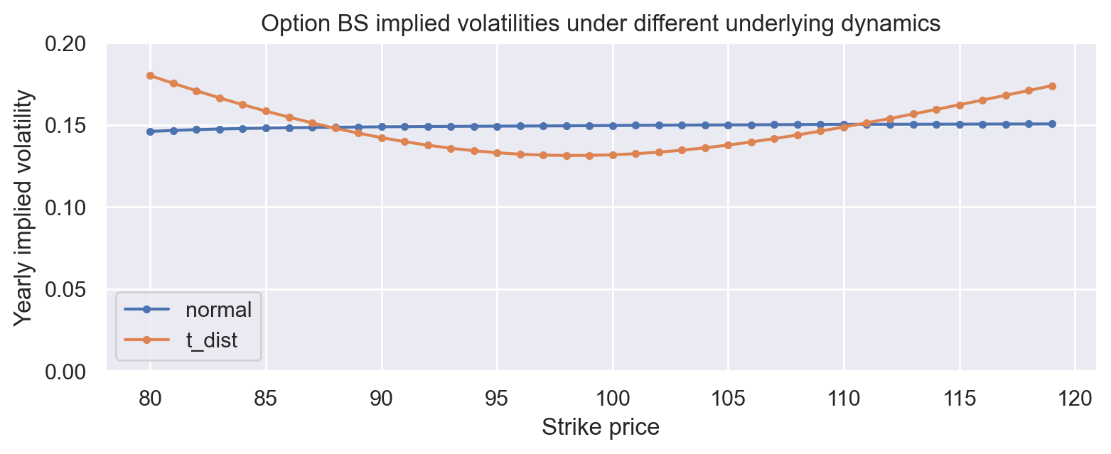
This notebook shows that the volatility smile is a caused by the excess kurtosis (the “fat tails”) of the log-returns distribution.

To show this we take three steps:

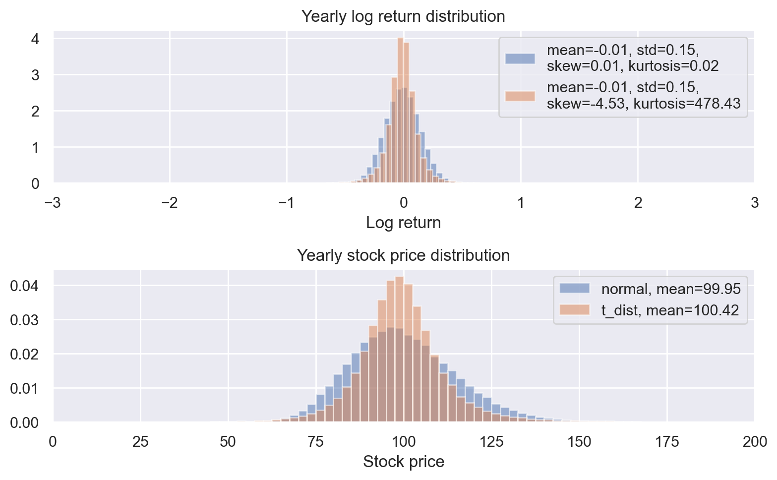
• Simulate the underlying prices using log-returns sampled from a normal distribution (thin-tailed) and a t-distribution (fat tailed).

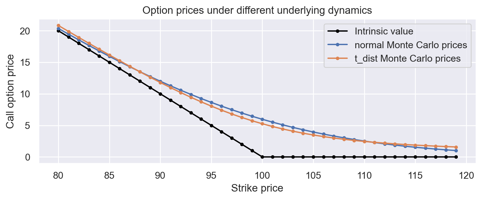
• For every distribution, compute the prices of a series of call options using samples of the underlying prices.

• For every distribution, compute the “implied volatility”, i.e. the volatility needed to make the Black Scholes model predictions match the observed price. This is done for every strike.

Log returns and stock prices

#| code-fold: true
%config InlineBackend.figure_format='retina'
import matplotlib.pyplot as plt
import numpy as np
import seaborn as sns

from numpy import newaxis
from scipy.stats import norm, skew, kurtosis
from scipy.optimize import minimize_scalar

plt.rcParams['figure.figsize'] = (9, 3)
sns.set_theme(style="darkgrid")

rng = np.random.default_rng(seed=42)

yearly_volatility = 0.15
initial_value = 100
num_samples = 100_000


def compute_normal_log_returns_and_stock_prices(
    yearly_volatility, initial_value, num_samples
):
    lognormal_mean_one_correction = -(yearly_volatility**2) / 2
    yearly_log_returns = rng.normal(
        loc=lognormal_mean_one_correction,
        scale=yearly_volatility,
        size=(num_samples,),
    )
    stock_price_samples = initial_value * np.exp(yearly_log_returns)
    return dict(
        yearly_log_returns=yearly_log_returns, stock_price_samples=stock_price_samples
    )


def compute_t_dist_log_returns_and_stock_prices(
    yearly_volatility, initial_value, num_samples, degrees_of_freedom
):
    lognormal_mean_one_correction = -(yearly_volatility**2) / 2
    # the variance of a t-distributed random variable is df / (df - 2) so to match it
    # with the Normal we need to add a correction factor.
    t_dist_std_correction = 1 / np.sqrt(degrees_of_freedom / (degrees_of_freedom - 2))
    yearly_log_returns = lognormal_mean_one_correction + yearly_volatility * (
        t_dist_std_correction
    ) * rng.standard_t(
        df=degrees_of_freedom,
        size=(num_samples,),
    )
    stock_price_samples = initial_value * np.exp(yearly_log_returns)
    return dict(
        yearly_log_returns=yearly_log_returns, stock_price_samples=stock_price_samples
    )


def compute_skewed_t_dist_log_returns_and_stock_prices(
    yearly_volatility, initial_value, num_samples, degrees_of_freedom
):
    lognormal_mean_one_correction = -(yearly_volatility**2) / 2
    # the variance of a t-distributed random variable is df / (df - 2) so to match it
    # with the Normal we need to add a correction factor.
    t_dist_std_correction = 1 / np.sqrt(degrees_of_freedom / (degrees_of_freedom - 2))
    yearly_log_returns = lognormal_mean_one_correction + yearly_volatility * (
        t_dist_std_correction
    ) * rng.standard_t(
        df=degrees_of_freedom,
        size=(num_samples,),
    )
    stock_price_samples = initial_value * np.exp(yearly_log_returns)
    return dict(
        yearly_log_returns=yearly_log_returns, stock_price_samples=stock_price_samples
    )

distributions = {
    "normal": compute_normal_log_returns_and_stock_prices(
        yearly_volatility, initial_value, num_samples
    ),
    "t_dist": compute_t_dist_log_returns_and_stock_prices(
        yearly_volatility, initial_value, num_samples, degrees_of_freedom=3
    ),
}

# | code-fold: true
def plot_log_return_and_stock_price(distributions):
    fig, (log_return_ax, stock_price_ax) = plt.subplots(
        nrows=2, ncols=1, figsize=(8, 5)
    )
    for name, dist in distributions.items():
        ylr = dist["yearly_log_returns"]
        log_return_ax.hist(
            ylr,
            bins=np.arange(ylr.min(), ylr.max(), 0.05),
            density=True,
            label=f"mean={ylr.mean():.2f}, std={ylr.std():.2f},\n"
            f"skew={skew(ylr):.2f}, kurtosis={kurtosis(ylr):.2f}",
            alpha=0.5,
        )
        log_return_ax.set_xlim(-3, 3)
    log_return_ax.set_xlabel("Log return")
    log_return_ax.set_title("Yearly log return distribution")
    log_return_ax.legend()
    for name, dist in distributions.items():
        sp = dist["stock_price_samples"]
        stock_price_ax.hist(
            sp,
            bins=np.arange(0, 200, 2.5),
            range=(-3, 3),
            density=True,
            label=f"{name}, mean={sp.mean():.2f}",
            alpha=0.5,
        )
        stock_price_ax.set_xlim(0, 200)
    stock_price_ax.set_xlabel("Stock price")
    stock_price_ax.set_title("Yearly stock price distribution")
    stock_price_ax.legend()
    fig.tight_layout()
    return fig


plot_log_return_and_stock_price(distributions)
None

Monte Carlo Option Pricing

def compute_call_prices_monte_carlo(stock_price_samples, strikes):
    return np.maximum(
        0,
        stock_price_samples[:, newaxis] - strikes[newaxis, :],
    ).mean(axis=0)


strikes = np.arange(80, 120, 1)

for dist in distributions.values():
    dist["call_prices"] = compute_call_prices_monte_carlo(
        dist["stock_price_samples"], strikes
    )

# | code-fold: true
def plot_monte_carlo_prices(distributions):
    fig, ax = plt.subplots(figsize=(9, 3))
    ax.plot(
        strikes,
        np.maximum(0, initial_value - strikes),
        label="Intrinsic value",
        marker=".",
        color="black",
    )
    for name, dist in distributions.items():
        ax.plot(
            strikes, dist["call_prices"], label=f"{name} Monte Carlo prices", marker="."
        )
    ax.set_xlabel("Strike price")
    ax.set_ylabel("Call option price")
    ax.legend()
    ax.set_title("Option prices under different underlying dynamics")
    return fig


plot_monte_carlo_prices(distributions)
None

Black-Scholes implied volatilities

def compute_call_price_black_scholes(S, t, sigma, r, K, T):
    tau = T - t
    N = norm.cdf

    d1 = (np.log(S / K) + (r + 0.5 * sigma**2) * tau) / (sigma * np.sqrt(tau))
    d2 = d1 - sigma * np.sqrt(tau)

    V = S * N(d1) - K * N(d2)

    return V


def value_to_iv(V, S, t, r, K, T):
    optimization_result = minimize_scalar(
        fun=lambda sigma: (
            (V - compute_call_price_black_scholes(S, t, sigma + 1e-9, r, K, T)) ** 2
        ),
        bounds=(0, 1),
    )
    assert optimization_result.success
    return optimization_result.x

for dist in distributions.values():
    dist["implied_volatilities"] = np.array(
        [
            value_to_iv(V=V, S=initial_value, t=0, r=0, K=K, T=1)
            for K, V in zip(strikes, dist["call_prices"])
        ]
    )

# | code-fold: true
def plot_implied_volatilities(distributions):
    fig, ax = plt.subplots(figsize=(9, 3))
    for name, dist in distributions.items():
        ax.plot(strikes, dist["implied_volatilities"], marker=".", label=f"{name}")
    ax.set_ylim(0, 0.2)
    ax.set_xlabel("Strike price")
    ax.set_ylabel("Yearly implied volatility")
    ax.legend()
    ax.set_title("Option BS implied volatilities under different underlying dynamics")
    return fig


plot_implied_volatilities(distributions)
None