Option Implied Stock Price Distributions
# | code-fold: true
import numpy as np
import pandas as pd
import QuantLib as ql
import seaborn as sns
import yfinance as yf
from scipy.optimize import minimize_scalar
from scipy.stats import norm
# | code-fold: true
import matplotlib.pyplot as plt

%config InlineBackend.figure_format='retina'
sns.set_theme(style="whitegrid")
plt.rcParams["figure.figsize"] = (9, 3)
plt.rcParams["axes.grid"] = True
plt.rcParams["lines.marker"] = "."
Introduction
Options are financial contracts that give the buyer the right to purchase (or sell) the underlying asset at a fixed price in a certain time period. The strike \(E\) of an option determines the price at which the underlying can be bought (for a call option) or sold (for a put option). The exiration \(T\) determines the date at which the contract stops being valid.
Option prices contain the market’s probabilistic forecast on the future price of the underlying. This is because, in theory, the value of a call option \(V(S, t)\) at time \(t\) on an underlying \(S\) is given by:
\[V(S, t) = e^{-r(T - t)} \mathbb{E}^{\mathbb{Q}} \left[ \text{max}(S - E, 0) \right]\]where \(\mathbb{E}^{\mathbb{Q}}[f(S)]\) is the expectation of a function of the underlying \(f(S)\) under the risk-neutral probability measure \(\mathbb{Q}\).
We can recover the distribution (or probability meausure) of future prices \(\mathbb{Q}\) by “inverting” the expectation that determines the option prices. How? In 1978 Breeden and Litzenberger gave us a formula that links option prices and the Probability Distribution Function (PDF) of the risk-netral distribution:
\[\frac{\partial^2 V}{\partial E^2} = e^{-r(T - t)} p^{\mathbb{Q}}(E)\]Method
Can we just use prices?
The simplest implementation applies the Breeden-Litzenberger formula directly to option prices by approximating the second-order derivative with finite differences:
\[\begin{align*} \frac{\partial^2 V}{\partial E^2} & = e^{-r(T - t)} p^{\mathbb{Q}}(E) \\ \implies p^{\mathbb{Q}}(E) & = e^{r(T - t)} \frac{\partial^2 V}{\partial E^2} \\ & \approx e^{r(T - t)} \frac{V(E + \delta E) + 2 V(E) - V(E - \delta E)}{(\delta E)^2} \end{align*}\]Unfortunately, the option’s strikes aren’t close enough to one another get a good approximation of the second derivative. For underlyings in the \(\$100-\$200\) range, the strikes are usually \(\$5\) apart from each other.
To improve the finite difference approximation we can interpolate the prices. Unfortunately this can lead to arbitrages, because a linear or, worse, a concave price interpolation implies a zero or negative (!) value in the implied future price PDF.
Let’s work in IV-space
Instead of directly interpolating the option’s prices, we take a step backwards and interpolate one of the parameters that determine the price of an option.
The price of an option is determined by several parameters, and the full formula is:
\[\text{option price} = V(S, t; \sigma, r, D, E, T)\]where:
- \(S\) is the price of the underlying asset
- \(t\) is the time to expiration (in years)
- \(\sigma\) is the volatility (annualized standard deviation of the returns) of the underlying
- \(r\) is the interest rate (annualized, compounded continuously)
- \(D\) is the dividend yield of the asset, e.g. a stock
- \(E\) is the strike price
- \(T\) is the expiration date
We choose to interpolate the volatility \(\sigma\). But wait, under the Black-Scholes (BS) model, isn’t the volatility constant? What does it mean to interpolate it? It turns out that in practice, option prices do not follow the Black-Scholes model exactly. Running an option trading desk that trust the BS model unconditionally is a fun experiment left for the reader (this is not investment advice).
By interpolating volatility we mean several steps:
- Using the option prices to compute the Implied Volatilities (IVs), i.e. the volatilities that make the BS model match the market prices
- Interpolating the IVs into a continuous curve, using some parametric or nonparametric model
- Using the interpolated IVs and the BS model to compute continuous prices for the options
After all of these steps we have continuous prices that we can use to estimate the price distribution via finite differences.
Implementation
Price
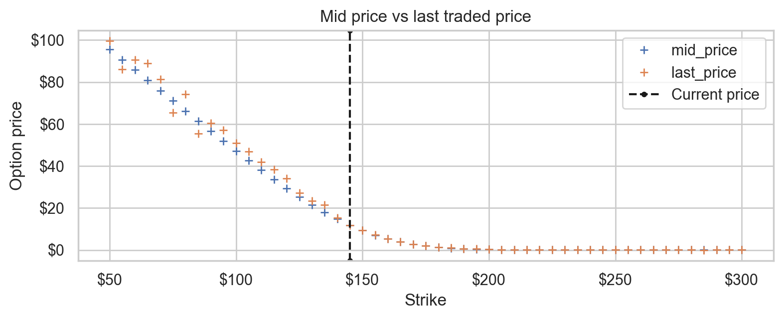
We use the Yahoo Finance API to download the prices of call options on Apple, expiring on February 17, 2023.
ticker = yf.Ticker("AAPL")
# | code-fold: true
def decorate_price_axes(ax: plt.Axes):
    ax.axvline(ticker.info["currentPrice"], ls="--", c="k", label="Current price")
    ax.xaxis.set_major_formatter("${x:.0f}")
    ax.yaxis.set_major_formatter("${x:.0f}")
    ax.legend()


def decorate_iv_axes(ax: plt.Axes):
    ax.axvline(ticker.info["currentPrice"], ls="--", c="k", label="Current price")
    ax.xaxis.set_major_formatter("${x:.0f}")
    ax.yaxis.set_major_formatter("{x:.0%}")
    ax.set_xlabel("Strike")
    ax.set_ylabel("Implied volatility")
    ax.legend()
prices = (
    ticker.option_chain(date="2023-02-17")
    .calls.rename(columns={"lastPrice": "last_price"})[
        ["strike", "bid", "ask", "last_price"]
    ]
    .assign(mid_price=lambda df: (df["bid"] + df["ask"]) / 2)
    .set_index("strike")[["mid_price", "last_price"]]
)
We estimate the prices using the midprice, the arithmetic mean of bid and ask. Using the last traded price for each option contract gives a much noisier estimate.
# | code-fold: true
ax = prices.plot(
    style="+",
    xlabel="Strike",
    ylabel="Option price",
    title="Mid price vs last traded price",
)
decorate_price_axes(ax)
None
Implied Volatility (IV)
We implement in call_option_value_black_scholes the Black-Scholes
formula for the price of an European call option:
\(V(S, t) = S e^{-D (T- t)} N(d_1) - E e^{-r (T- t)} N(d_2)\) \(d_1 = \frac{ \log(S / E) + \left(r + \frac{\sigma^2}{2}\right) (T - t) }{ \sigma \sqrt{T - t} }\) \(d_2 = d_1 - \sigma \sqrt{T - t}\)
def call_option_value_black_scholes(S, t, sigma, r, D, E, T,):
    tau = T - t
    N = norm.cdf

    d1 = (np.log(S / E) + (r + 0.5 * sigma**2) * tau) / (sigma * np.sqrt(tau))
    d2 = d1 - sigma * np.sqrt(tau)

    V = S * np.exp(-D * tau) * N(d1) - E * np.exp(-r * tau) * N(d2)

    return V
Then, we implement in value_to_iv the “inverse” of this formula. This
function goes from the price of an European call option to the implied
volatility that makes the BS formula match the market price.
If you like formulas, this is the optimization problem that is being solved:
\[\sigma = \underset{\tilde \sigma}{\mathrm{argmin}} (V^{\text{market}} - V^{BS}(\tilde \sigma))^2\]def value_to_iv(V, E, S, t, r, D, T):
optimization_result = minimize_scalar(
fun=lambda sigma: (
V - call_option_value_black_scholes(S, t, sigma + 1e-3, r, D, E, T)
)
** 2,
bounds=(0, float("+inf")),
)
assert optimization_result.success
return optimization_result.x
S = ticker.info["currentPrice"]
r = 0.0325
D = 0.0059
T = 1.0
today = ql.Date(31, 10, 2022)
expiration = ql.Date(17, 2, 2023)
trading_days = 252
t = (trading_days - ql.TARGET().businessDaysBetween(today, expiration)) / (trading_days)
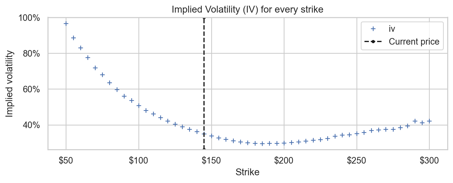
ivs = pd.DataFrame(index=prices.index)
ivs["iv"] = [
value_to_iv(V, E, S, t, r, D, T) for E, V in zip(prices.index, prices["mid_price"])
]
We plot the volatility surface, the implied volatility for every strike. First, we notice that the volatility is not constant, instead it has a “smile-like” shape, implying that deep out-of-the money tails are more expensive than the BS model predicts. Second, there seem to be some outliers in the sub $100 strikes.
# | code-fold: true
ax = ivs.plot(title="Implied Volatility (IV) for every strike", style="+")
decorate_iv_axes(ax)
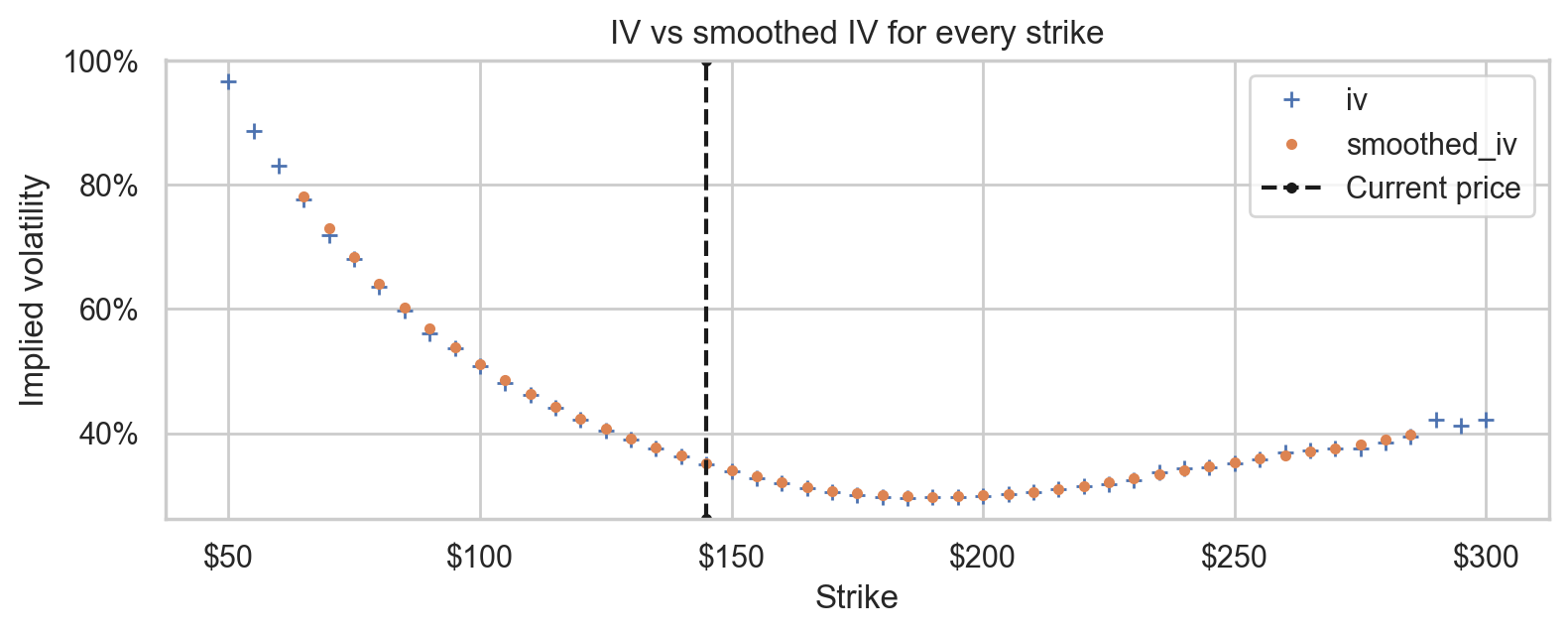
Smoothed IV
smoothed_ivs = (
    ivs
    .rolling(window=7, center=True, win_type="gaussian")
    .mean(std=2)
    .dropna()
    .rename(columns={"iv": "smoothed_iv"})
)
# | code-fold: true
ax = ivs.plot(title="IV vs smoothed IV for every strike", style="+")
smoothed_ivs.plot(ax=ax, style=".")
decorate_iv_axes(ax)
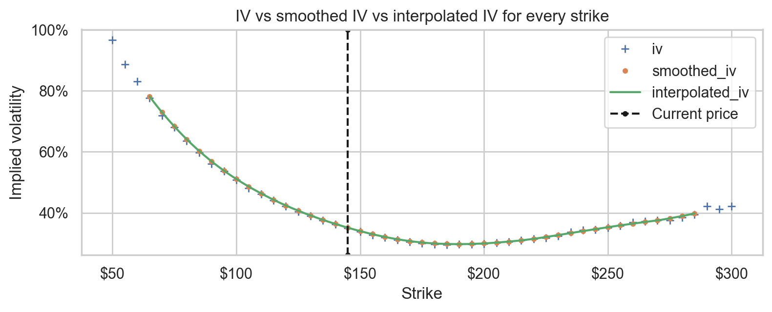
Interpolated IV
Then, we intepolate between the smoothed IVs using a cubic spline.
upsampling_rate = 50
interpolated_ivs = smoothed_ivs.reindex(
    np.linspace(
        smoothed_ivs.index.min(),
        smoothed_ivs.index.max(),
        (smoothed_ivs.index.size - 1) * upsampling_rate + 1,
    )
).assign(
    interpolated_iv=lambda df: df["smoothed_iv"].interpolate(method="cubicspline")
)[
    ["interpolated_iv"]
]
# | code-fold: true
ax = ivs.plot(style="+", title="IV vs smoothed IV vs interpolated IV for every strike")
smoothed_ivs.plot(ax=ax, style=".")
interpolated_ivs.plot(ax=ax, style="-")
decorate_iv_axes(ax)
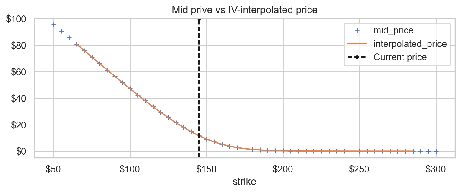
IV-Interpolated price
interpolated_prices = pd.DataFrame(index=interpolated_ivs.index)
interpolated_prices["interpolated_price"] = [
    call_option_value_black_scholes(S, t, sigma, r, D, E, T)
    for E, sigma in zip(interpolated_ivs.index, interpolated_ivs["interpolated_iv"])
]
# | code-fold: true
ax = prices[["mid_price"]].plot(style="+", title="Mid prive vs IV-interpolated price")
interpolated_prices.plot(style="-", ax=ax)
decorate_price_axes(ax)
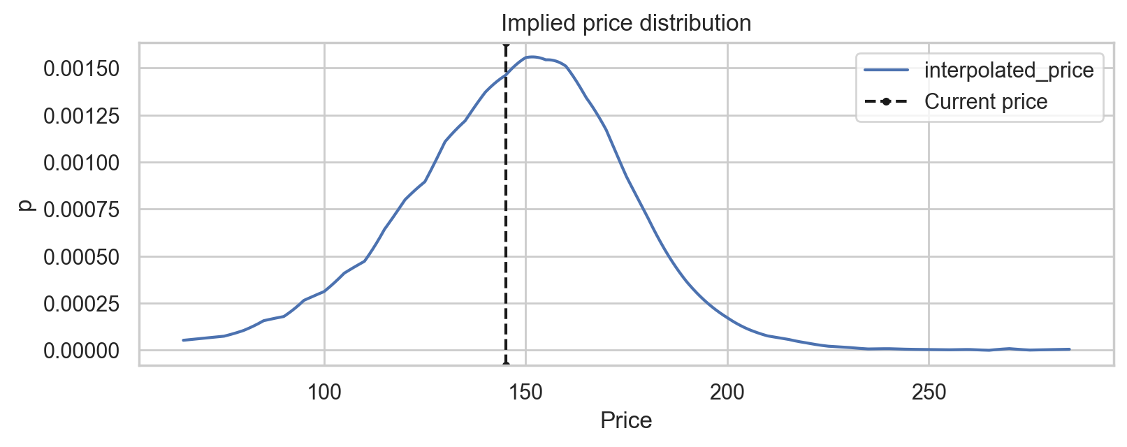
Implied price PDF
implied_price_pdf = interpolated_prices.pipe(
    lambda df: df.shift(-1) - 2 * df + df.shift(1)
).dropna().transform(lambda df: df / df.sum())
# | code-fold: true
ax = implied_price_pdf.plot(
    style="-", xlabel="Price", ylabel="p", title="Implied price distribution"
)
ax.axvline(ticker.info["currentPrice"], ls="--", c="k", label="Current price")
ax.legend()
None
Conclusion and future work
TODO(Andrea): write
References
- Paul Wilmott Introduces Quantitative Finance, 2nd Edition
- Breeden, Litzenberger - Prices of State-Contingent Claims Implicit in Option Prices
- Reasonable Deviations - Option-implied probability distributions, part 2
- Morgan Stanley - How Options Implied Probabilities Are Calculated
- Quant StackExchange - Explaining the Risk Netural Measure