A probabilistic programming language in 70 lines of Python
Full code available at github.com/mrandri19/smolppl
The continuation to this post, called “Predictive sampling and graph traversals” is now available!
Introduction
In this post I will explain how Probabilistic Programming Languages (PPLs) work by showing step-by-step how to build a simple one in Python.
I expect the reader to be moderately familiar with PPLs and Bayesian statistics, as well as having a basic understanding of Python. They could be, for example, statisticians/AI researchers/or curious programmers.
At the end, we will have built an API like this one:
mu = LatentVariable("mu", Normal, [0.0, 5.0])
y_bar = ObservedVariable("y_bar", Normal, [mu, 1.0], observed=3.0)

evaluate_log_density(y_bar, {"mu": 4.0})
This first two lines define the probability model
\[\mu \sim \text{Normal}(0, 5)\] \[\bar y \sim \text{Normal}(\mu, 1)\]and the last line evaluates, at \(\mu = 4\), the (unnormalized) probability distribution defined by the model, conditioned on the data \(\bar y = 3\).
\[\log p(\mu = 4 | \bar y = 3)\]My hope is to give the reader an understanding of how PPLs work behind the scenes as well as an understanding of Embedded Domain-Specific Languages (EDSLs) implementation in Python.
Related work
As far as I know, there are no simple, didactic implementations of PPLs in Python.
The book “The Design and Implementation of Probabilistic Programming Languages” is focused on programming language theory, requiring familiarity with continuation-passing style and coroutines, as well as using JavaScript as their implementation language. The blog post “Anatomy of a Probabilistic Programming Framework” contains an great high-level overview, but does not delve into implementation details or shows code samples. Finally, Junpeng Lao’s talk and PyMC3’s Developer guide describe in detail the implementation details of PyMC, but it is not straightforward to implement a PPL just based on those.
Update: another great overview is chapter 10 of Bayesian Modeling and Computation in Python.
Implementation
High-level representation
We will use this model throughout the process as our guiding example.
\[\mu \sim \text{Normal}(0, 5)\] \[\bar y \sim \text{Normal}(\mu, 1)\]These expressions define a joint probability distribution with an associated Probability Density Function (PDF):
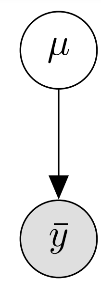
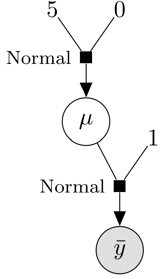
\[p(\mu, \bar y) = \text{Normal}(\mu | 0, 5) \text{Normal}(\bar y | \mu, 1)\]We can represent this expression (and the model) graphically in two ways: graphical models and directed factor graphs.


While PGMs are more common in the literature, I believe that directed factor graphs are more useful for a PPL implementer. The graph tells us several aspects of our representation:
- We need a way to represent two types of variables:
- ones of which we know the observed value (\(\bar y\), gray background)
- and ones which are latent and cannot be observed (\(\mu\), white background).
- We need to handle constants and the distribution of each variable.
- Finally, we need a way to connect together observed variables, latent variables, and constants.
Distributions
For our purposes, a distribution is class with a function that can evaluate its
log probability density function at a point.
The log_density function takes a float representing a point in the
distribution’s support, a List[float] of the distribution’s parameters,
and returns a float equal to the log-PDF evaluated at the point.
To implement new distributions we will inherit from the Distribution abstract
class.
We will not support vector or matrix-valued distributions for now.
Using SciPy we implement the Normal distribution, with param[0] being the
mean and param[1] the standard deviation.
from scipy.stats import norm


class Distribution:
    @staticmethod
    def log_density(point, params):
        raise NotImplementedError("Must be implemented by a subclass")


class Normal(Distribution):
    @staticmethod
    def log_density(point, params):
        return float(norm.logpdf(point, params[0], params[1]))
Variables and DAGs
Let us now focus our attention on variables. Three aspects characterize them: they have an associated distribution, they can be latent or observed, and they are linked to one another (i.e they can have children).
The dist_class field is a Distribution associated with the variable.
When evaluating the full log density, we will use this field to access the
log_density method of the variable’s distribution.
We differentiate latent from observed variables using the classes
LatentVariable and ObservedVariable.
Observed variables have an observed field with the observed value.
Since latent variables do not have a value at model-specification time, we will
have to give them a value at runtime, while evaluating the full log density.
To specify the runtime value of latent variables we use need to identify them
with a unique string name.
Finally, we can make the parameters of a variable’s distribution be variables or
constants.
In our example, the mean of \(\bar y\) is \(\mu\) a Normal random variable,
while its standard deviation is the constant \(1\).
To represent this we use the dist_args property.
The mypy signature of dist_args is
dist_args: Union[float, LatentVariable, ObservedVariable].
This means that a latent/observed variable can have “arguments” which themselves
are latent/observed variables of constants, thus creating a
Directed Acyclic Graph (DAG).
class LatentVariable:
    def __init__(self, name, dist_class, dist_args):
        self.name = name
        self.dist_class = dist_class
        self.dist_args = dist_args


class ObservedVariable:
    def __init__(self, name, dist_class, dist_args, observed):
        self.name = name
        self.dist_class = dist_class
        self.dist_args = dist_args
        self.observed = observed
We can visualize the DAG and notice a key difference from the latent factor graph representations: the arrows are reversed. This is a consequence of how we specify the variables in our modeling API, and it turns out that having the observed variable as the root is also a better representation for computing the joint log density.


To further clarify, let’s see what the dist_args for our model look like:
mu = LatentVariable("mu", Normal, [0.0, 5.0])
y_bar = ObservedVariable("y_bar", Normal, [mu, 1.0], observed=5.0)

print(mu)
# => <__main__.LatentVariable object at 0x7f14f96719a0>
print(mu.dist_args)
# => [0.0, 5.0]
print(y_bar)
# => <__main__.ObservedVariable object at 0x7f14f9671940>
print(y_bar.dist_args)
# => [<__main__.LatentVariable object at 0x7f14f96719a0>, 1.0]
Evaluating the log density
We are almost done, the missing piece is a way to evaluate the joint log-density using our DAG. To do it we need to traverse the DAG, and add together the log-densities of each variable. Adding log densities is equal to multiplying the densities, but it is a lot more numerically stable.
To traverse the DAG we use a recursive algorithm called
depth-first search.
The collect_variables function visits all variables once, collecting all
non-float variables into a list.
The algorithm starts from the root, and then recursively visits all dist_args
to collect each variable.
def evaluate_log_density(variable, latent_values):
    visited = set()
    variables = []

    def collect_variables(variable):
        if isinstance(variable, float):
            return

        visited.add(variable)
        variables.append(variable)

        for arg in variable.dist_args:
            if arg not in visited:
                collect_variables(arg)

    collect_variables(variable)
For each variable we need to obtain a numeric value for each one of its
arguments, and using them evaluate the distribution’s log density.
float arguments are already numbers, LatentVariables take different values
depending on where we wish to evaluate the log density.
To specify the values of the latent variables we pass a dictionary of variable
name to numbers, called latent_values.
Notice how ObservedVariables cannot be arguments, they can only be roots.
N.B.
dist_argscan befloatconstants orLatentVariables.
dist_paramsare allfloats, either constants or values we assigned to the latent variables vialatent_valuesat runtime (i.e. when we actually compute the log density).
Finally, with the distribution’s parameters extracted from the arguments, we
can update the total log density.
LatentVariables need to evaluate the log density at the point specified in
latent_values while ObservedValues evaluate the log density at the point
specified in observed.
    log_density = 0.0
    for variable in variables:
        dist_params = []
        for dist_arg in variable.dist_args:
            if isinstance(dist_arg, float):
                dist_params.append(dist_arg)
            if isinstance(dist_arg, LatentVariable):
                dist_params.append(latent_values[dist_arg.name])

        if isinstance(variable, LatentVariable):
            log_density += variable.dist_class.log_density(
                latent_values[variable.name], dist_params
            )
        if isinstance(variable, ObservedVariable):
            log_density += variable.dist_class.log_density(
                variable.observed, dist_params
            )

    return log_density
Let’s check that the total log probability is equal to what we expect
mu = LatentVariable("mu", Normal, [0.0, 5.0])
y_bar = ObservedVariable("y_bar", Normal, [mu, 1.0], observed=5.0)

latent_values = {"mu": 4.0}
print(evaluate_log_density(y_bar, latent_values))
# => -4.267314978843446
print(norm.logpdf(latent_values["mu"], 0.0, 5.0)
    + norm.logpdf(5.0, latent_values["mu"], 1.0))
# => -4.267314978843446
Conclusion and future work
Distributions, variable DAGs, and log density evaluation are the components of a probabilistic programming language. The variables can be latent, observed, or constants and each one must be handled separately in the log density calculation. We implement these concepts in Python leading to a simple but powerful PPL.
The next steps would be to add support for tensors and transformations of random variables, in order to support more useful models like linear regression and hierarchical/mixed effects models. Another useful feature would be to build an API for prior predictive sampling, Finally, instead of doing the calculations in python, using a compute graph framework like theano/aesara, JAX, or TensorFlow would be greatly beneficial to the performance. A computation graph would also allow to calculate the gradient of the log density via reverse-mode automatic differentiation which is needed for advanced samplers like Hamiltonian Monte Carlo.
Bonus: posterior grid approximation
We have not talked about what the log density is useful for. One example would be to find the mode of the posterior distribution, i.e. finding the most likely value for our parameters.
In this case the observed sample mean is \(1.5\), which will be moved a little towards \(0\) by the Normal zero-mean prior. This means that the Maximum A Posteriori (MAP) estimate will be around \(1.4\).
import numpy as np
import pandas as pd
import altair as alt

from smolppl import Normal, LatentVariable, ObservedVariable,
                    evaluate_log_density

# Define model
# Weakly informative mean prior
mu = LatentVariable("mu", Normal, [0.0, 5.0])

# Observation model. I make some observations y_1, y_2, ..., y_n and compute the
# sample mean y_bar. It is given that the sample mean has standard deviation 1.
y_bar = ObservedVariable("y_bar", Normal, [mu, 1.0], observed=1.5)

# Grid approximation for the posterior
# Since the prior has mean 0, and the observations have some uncertainty, I
# expect the mode to be a bit smaller than 1.5. Something like 1.4
grid = np.linspace(-4, 4, 20)
evaluations = [evaluate_log_density(y_bar, {"mu": mu}) for mu in grid]

# Plotting
data = pd.DataFrame({"grid": grid, "evaluations": evaluations})
chart = alt.Chart(data).mark_line(point=True).encode(
    x=alt.X('grid', axis=alt.Axis(title="mu")),
    y=alt.Y('evaluations', axis=alt.Axis(title="log density"))
).interactive().configure_axis(
    labelFontSize=16,
    titleFontSize=16
)
chart